In today’s cloud-driven landscape, cost optimization is critical to managing infrastructure efficiently. As organizations increasingly adopt containerized environments like Google Kubernetes Engine (GKE) for their workloads, understanding how to optimize costs within these environments becomes paramount. GKE, Google Cloud’s managed Kubernetes service, provides a range of built-in features and tools to help users maximize resource utilization and minimize unnecessary expenses. The last article, “The Challenges and Strategies of Managing Kubernetes Costs,” gives an overview of the theme. In this article, we go deeper into configuring the GCP console to best cost management.
In this article, we delve into the realm of cost optimization in GKE, exploring the various strategies and techniques employed to streamline resource allocation and achieve better efficiency. We will uncover the power of leveraging GKE’s Cost Optimization tab, which offers insightful visualizations and data per workload, enabling you to analyze usage patterns, adjust requests and limits, and identify areas for improvement. Additionally, we will explore Vertical Pod Autoscaler’s (VPA) benefits and its role in rightsizing workloads based on historical and current usage.
Imagine you have a refrigerator in your kitchen. The refrigerator represents your GKE cluster, and the items inside it represent the workloads running on the cluster. Just like you want to keep your refrigerator organized and minimize waste, you want to optimize your GKE cluster to ensure efficient resource utilization and cost savings.
In this analogy, the configuration settings act as your control over the refrigerator’s temperature and storage compartments. Similarly, in GKE, the configurations, such as requests and limits, allow you to define the amount of resources (CPU and memory) allocated to each workload.
By setting appropriate requests and limits for your workloads, you can ensure they have enough resources to operate efficiently without wasting excess resources. It’s like storing the right amount of food in each refrigerator compartment so nothing goes to waste or causes overcrowding.
Additionally, the Cost Optimization tab in GKE is like having a transparent glass door on your refrigerator, enabling you to see and analyze the usage patterns of each workload. Just as you can visually assess which items in your refrigerator are taking up more space, the Cost Optimization tab provides visualizations and data that help you identify workloads that might be over or underutilizing resources.
By adjusting the configurations based on the insights from the Cost Optimization tab, you can optimize resource allocation, avoid resource conflicts (like items fighting for space in the refrigerator), and ultimately achieve significant cost savings, just as you would minimize food waste and save money by efficiently managing your refrigerator.
Hey ho, let’s go!
1. Understanding Configurations in GKE
Once you’re on the Kubernetes clusters page or the details page of a specific cluster, you can perform various tasks such as viewing cluster information, managing node pools, deploying applications, scaling resources, configuring networking, and more.
1.1 Navigating to Kubernetes Engine if you’re a new user:
- Open a web browser and go to the GCP Console website: https://console.cloud.google.com/.
- Sign in to your Google account associated with the GCP project that contains the Kubernetes clusters. Ensure that you have the necessary permissions to access and manage the clusters.
- Once you’re signed in, you’ll be redirected to the GCP Console dashboard.
- You’ll find a navigation menu on the left side of the GCP Console dashboard. Scroll down and locate the “Kubernetes Engine” section. Expand it by clicking on the arrow next to the section name.
- Click on “Kubernetes clusters” under the “Kubernetes Engine” section. This will take you to the Kubernetes clusters page.
- On the Kubernetes clusters page, you’ll see a list of all the Kubernetes clusters in your GCP project.
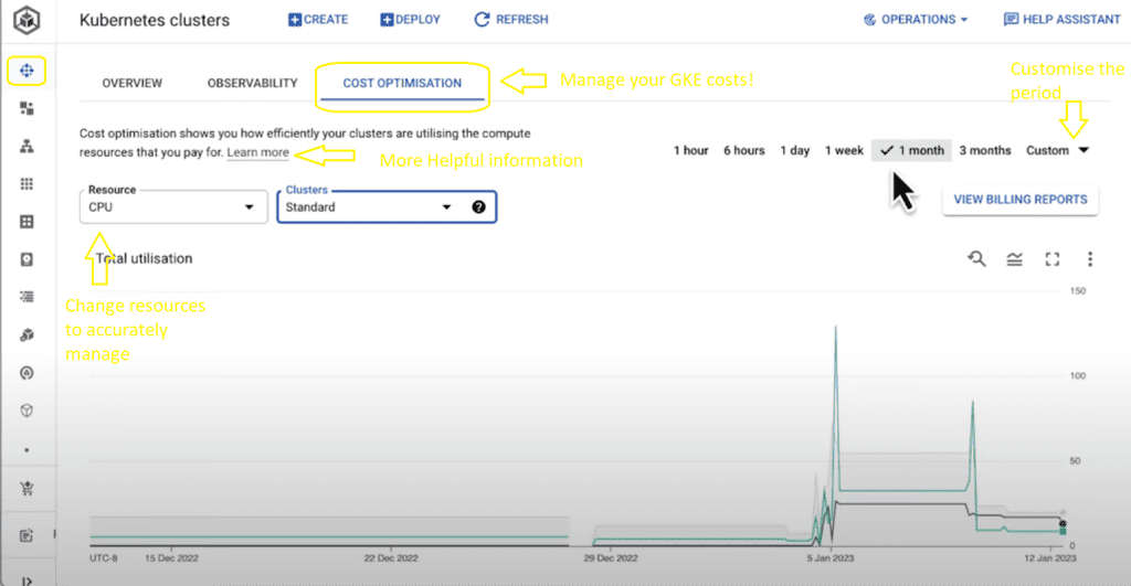
- You now have the option: “Cost optimization.”
Remember, you need the appropriate permissions and roles assigned to your GCP account to access and manage Kubernetes clusters in your project. If you encounter permission issues, contact your project’s administrator or the person responsible for managing GCP access in your organization.
In this tab, we can see a time series visualization for our GKE clusters, which will get detailed information about resources across clusters in a project, starting with CPU across all standard clusters. For any given time over a customizable time window, in this case, one month, we can see the total allocated CPU across all of our standard clusters, the amount of CPU requested by pods running in those clusters, and the amount of CPU used by these pods.
We can also see the bar charts below to show us what usage, requests, and allocatable resources looked like over that defined time window.
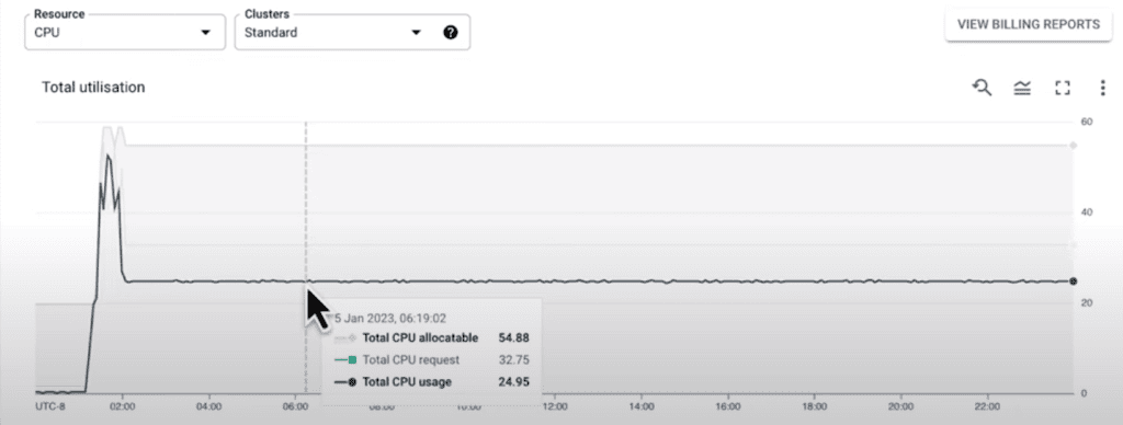
Now this information can help us understand how efficiently we bin pack our workloads onto nodes in our cluster. But what it can also do is give us insight into scaled-down efficiency. For example, we can use the time filter to look at a specific window in which we had a scale-up event. So let’s take a look at this example:

Scroll down, and now we can see that while we added nodes during the scale-up of pod requests, we could have gotten better cluster utilization by prioritizing scale-down after usage had stabilized. Information like this can help us make optimization-centric decisions like implementing the optimized utilization profile for Cluster Autoscaler, which was not enabled in our cluster during this time window. A change like that will not only help Cluster Autoscaler spin down under-utilized nodes better, but it’ll also give preference to scheduling pods on nodes with more usage to improve cluster bin packing. You can receive insights about optimizes:

We can also get the exact visualization from memory across our standard clusters. In this case, we can see that our clusters still have a bunch of unallocated memory. With this data, we can think about optimization decisions like choosing machine types with less memory in our clusters.
The time series visualization also supports GKE Autopilot clusters. Chance the option inside the field “Clusters”

One of the core differences between GKE Standard mode and GKE Autopilot mode is that Google manages your underlying node infrastructure in Autopilot. Thus, it handles the allocated resources for you in the cluster. So in this model, you don’t pay for infrastructure used or idle, but you pay for your pod requests. Thus, our optimization efforts focus on whether pods use their requested resources. As you can see, there is an opportunity to perform workload rightsizing across both memory and CPU. That is adjusting pod requests to reduce resource waste while still requesting what the pod needs to function.
Not only does this Cost Optimization tab show us data on resource utilization across clusters, but it also links us directly to its financial implications, as each cluster I’ve shown you here has GKE cost allocation enabled, which is integrated with Cloud billing.
When we click View Billing Reports, we’re navigated to Cloud billing with information about the cost of our clusters. However, in many cases, clusters house many workloads across multiple teams. What if we want to understand costs at a more granular level that can help us identify areas to optimize? With GKE cost allocation, we can filter billing data down to the cost of pod requests by namespace or labels across our clusters, in this case, some filtering based on namespaces. This is another reason to double-check that you’re using namespaces and labels to organize and identify teams and services in your clusters logically.
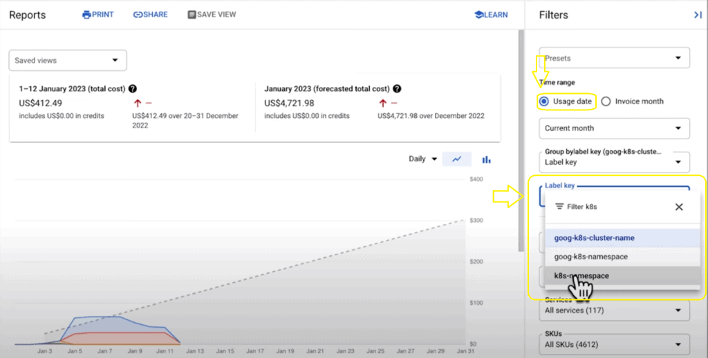
The “View Billing Reports” option in GKE allows us to access Cloud billing information related to the cost of our clusters. However, when dealing with clusters that house multiple workloads across different teams, we often need a more detailed understanding of costs to identify areas for optimization.
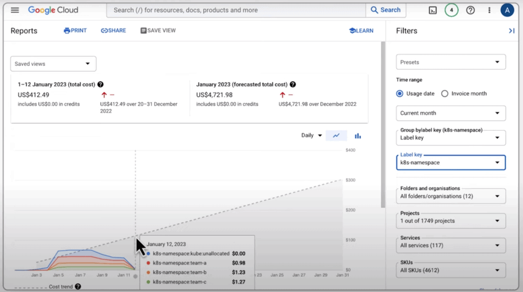
GKE cost allocation comes to our rescue by enabling us to filter billing data based on specific criteria, such as pod requests by namespace or labels. This level of granularity helps us analyze costs at a more fine-grained level, providing insights into how resources are allocated within clusters. It is crucial to ensure that namespaces and labels are effectively used to organize and identify teams and services in clusters logically.
Furthermore, GKE cost allocation also allows us to see the cost of unallocated resources within the cluster. This data can be exported to BigQuery, providing even more flexibility for analysis. Notably, the billing data encompasses all Google Cloud Platform (GCP) resources, not just GKE, enabling us to perform SQL queries to evaluate not only the cost of team workloads in GKE but also the associated backing and stateful services outside of GKE, such as Cloud Memorystore and Cloud SQL. This comprehensive view aids in optimizing costs across the entire infrastructure.
Once we have reviewed the macro-level information, diving deeper and analyzing the cost optimization data more granularly is essential. To do this, we navigate to the “Cost Optimization” tab in the Workload section of the GKE Console.

To simplify our analysis, we filter the view to focus on our standard cluster. This tab provides valuable insights into cost optimization for each workload. We can understand how workload usage relates to resource requests and limits over a defined time window through time series and bar graph visualizations.

Let’s examine each workload individually, starting with our alpha workload. This workload utilizes approximately 50% of its requested resources but only a quarter of its memory resources. This presents an opportunity to reduce resource requests, particularly in terms of memory potentially.
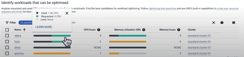
Moving on to our beta workload, we observe that it utilizes around 50% of its CPU requests. However, its memory usage exceeds the requested amount, as indicated by the yellow bar graph. This indicates an opportunity to increase the resource requests and set a limit for memory. Without limits, this workload may consume excessive memory on the node, leading to potential out-of-memory issues for other workloads sharing the same node. Remember, the best practice is to set memory limits for consumption and all budgets to GKE, and you can see this configuration in the field called “Limit” with the gray ball.

Our delta workload is an unfortunate example of a common problem where workloads are not configured with resource requests or limits. This leads to the same issue of noisy neighbors, where these workloads consume excessive resources on a node. Moreover, this lack of resource configuration hampers efficient cluster bin packing, as the cluster can only optimize resource allocation based on the provided requests.
On the other hand, we have the gamma workload, which presents an opportunity to increase the CPU resource request amount. By adjusting the CPU resource request, we can ensure that the workload receives adequate resources to operate efficiently.
But we can also observe from the memory usage of the workload that the bar graph reflects the appropriate limits that have been set. In this case, the limit is represented by the gray color. This data provides valuable insights for implementing cost optimization strategies.
Implementing cost optimization requires a cultural shift where cluster administrators collaborate with service owners to adjust resource requests. This helps correct issues and establishes best practices and standards for future demands and limits.
By working together, GKE facilitates team communication and collaboration, ensuring that relevant information surfaces and enables effective workload management.
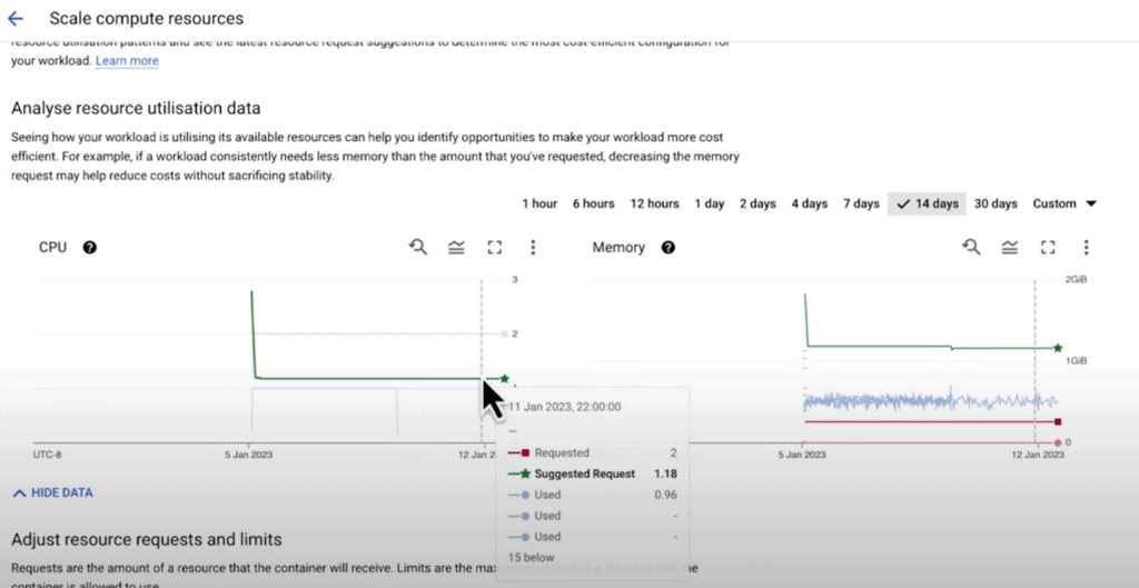
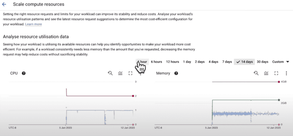
Now let’s examine our beta workload, where we can find recommendations directly from the Vertical Pod Autoscaler (VPA) in the GKE Console.

VPA’s recommendations are generated based on the workload’s historical and current usage patterns. To access these recommendations, navigate to the Actions menu and select “Scale,” followed by “Edit Resource Requests.” Make sure that HPA and VPA policies don’t clash if you don’t know about these mechanisms.
Imagine you’re hosting a party at your house and have a bunch of chairs set up for your guests. As more people arrive, you must add more chairs to accommodate everyone. Similarly, as people leave the party, you can remove some chairs to free up space.
In Kubernetes, Horizontal Pod Autoscaler (HPA) works like the magical chair provider. It automatically adds or removes your pod’s replicas based on your workload’s demand. So, when your workload becomes busier, more pods are created to handle the increased traffic. And when the demand decreases, some pods are automatically removed to optimize resource usage and save costs. HPA suits stateless (like a chair) and stateful (like a person) applications.
Now, let’s talk about Vertical Pod Autoscaler (VPA). Imagine you have a room with adjustable tables and chairs. VPA is like a clever assistant who observes the actual usage of these resources and adjusts their allocation accordingly. If the room is crowded and people need more space, the assistant expands the tables and chairs to accommodate the growing needs. And when the room becomes less crowded, the assistant can shrink the tables and chairs to save space and optimize resource allocation. VPA is beneficial for workloads that experience temporary high utilization.
Lastly, we have Cluster Autoscaler. Imagine you have a parking lot with flexible parking spots. Cluster Autoscaler is like an intelligent parking attendant who dynamically adjusts the number of available parking spots based on the number of cars coming in and going out. If the parking lot gets crowded, the attendant adds more parking spots to accommodate the increasing number of vehicles. And if the number of cars decreases, some parking spots are removed to save space and reduce costs. Similarly, Cluster Autoscaler adjusts the number of nodes in your cluster to match the current utilization, helping you optimize resource allocation and manage costs effectively.
So, these autoscaling tools in Kubernetes (HPA, VPA, and Cluster Autoscaler) work together to ensure your applications have the right amount of resources at the right time, just like chairs, tables, and parking spots are dynamically adjusted to meet the demands of your guests or cars.

We encounter green lines marked with star icons in the resource request editing interface. These represent the recommended values for CPU and memory requests. In the case of our beta workload, its memory usage exceeds the current requests. Therefore, the VPA recommendation suggests increasing the memory requests to better align with the workload’s needs.

Now, let’s shift our focus to the alpha workload. In the case of workloads with Horizontal Pod Autoscaler (HPA) based on a CPU usage threshold, changing CPU requests in isolation can have unintended consequences. Therefore, no specific recommendation is provided for CPU requests. However, there is still a recommended value for memory requests, which can aid teams in optimizing workload sizes for better cluster performance.

The functionality discussed thus far is highly beneficial for teams already utilizing GKE clusters. However, what about those just starting with GKE and prioritizing cost optimization? The GKE Console offers assistance for such users as well.

For beginners creating their first GKE cluster, there are helpful features available. One such feature is the setup guide for a cost-optimized GKE standard cluster. This guide provides a wizard-like experience, allowing users to create their clusters using a pre-defined template in the user interface (UI). This way, users can ensure that their GKE cluster is set up for success and optimized.

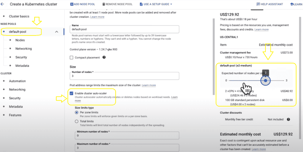
To simplify creating a cost-optimized GKE cluster, a template that incorporates many of the concepts discussed thus far is available. This template includes cluster autoscaling with an optimized utilization profile, Vertical Pod Autoscaling, and GKE cost allocation. However, the template is flexible, allowing users to make specific adjustments according to their cluster’s requirements.

If you prefer a more hands-on approach using the GKE Console, you can configure your cluster step by step. Throughout the configuration process, the Console estimates your cluster’s potential cost as you customize it. Additionally, suppose you plan on utilizing auto-scaling for your cluster. In that case, a slider is available to provide insights into the range of costs that may occur as the cluster dynamically adjusts based on demand. These tools help you make informed decisions and manage your cluster’s costs effectively.
Optimizing your GKE clusters is not a one-time task but an ongoing effort that involves collaboration among various team members. Cluster admins, workload owners, and billing managers are crucial in this process.
Throughout this exploration, we have witnessed the array of built-in features that GKE offers to assist you on your optimization journey. These features are designed to help you make informed decisions, identify improvement areas, and enhance your GKE clusters’ performance.
Remember, optimization is a continuous process. As new workloads are added, and existing ones evolve, it’s important to reassess and refine your cluster configurations regularly. By leveraging the tools and capabilities provided by GKE, you can proactively optimize your clusters, improve efficiency, and achieve better resource utilization.
So, embrace the collaborative effort, utilize the available features, and keep optimizing your GKE clusters to ensure they meet the evolving needs of your applications and deliver optimal performance.
This article explored various aspects of managing and optimizing Google Kubernetes Engine (GKE) clusters. From accessing and managing clusters to visualizing resource utilization and cost allocation, we delved into essential practices for efficient cluster management. We also discussed cost optimization techniques and how to create cost-optimized GKE clusters. But you don’t know the most important question: Why did the Kubernetes cluster start practicing yoga?
Because it wanted to find its inner container!
Sorry, with cost optimization, your sense of humor goes downs some levels and standards. I hope your GKE costs can do the same, lol.
Now that we’ve had “fun,” it’s time to gear up for the next article. Stay tuned for our next installment and continue your journey to become a cost optimization expert. May your pods always be scheduled and your deployments always be successful!
Until next time, happy optimizing!
o/